Linear Transformations
What does a linear transformation do to vectors?
Algebraic view
Recall that a linear transformation is a linear mapping between two vector spaces \(V\) and \(W\):
\[ \begin{equation*} T:V\rightarrow W \end{equation*} \]
What makes \(T\) linear are these two properties:
- \(T(\mathbf{v}_1 + \mathbf{v}_2) = T(\mathbf{v}_1) + T(\mathbf{v}_2)\), for all \(\mathbf{v}_1, \mathbf{v}_2 \in V\)
- \(T(c \cdot \mathbf{v}) = c \cdot T(\mathbf{v})\), for all \(c \in \mathbb{R}\) and \(\mathbf{v} \in V\)
In this course, we will be dealing with \(\mathbb{R}^{n}\). So, our transformations will be of the form: \[ \begin{equation*} T:\mathbb{R}^{n}\rightarrow \mathbb{R}^{m} \end{equation*} \]
To get a better idea about what a linear transformation does, let us restrict our attention to a map from \(\mathbb{R}^{2}\) to itself. If \(\mathbf{u}\) is a vector in \(\mathbb{R}^{2}\), then the transformation returns another vector in the same space. We can associate a matrix with every linear transformation. Assuming that we use the standard ordered basis \(\beta =\{\mathbf{e}_{1} ,\mathbf{e}_{2} \}\) for \(\mathbb{R}^{2}\) and calling the matrix \(\displaystyle \mathbf{T}\), we have:
\[ \begin{equation*} \mathbf{T} :=[T]_{\beta }^{\beta } =\begin{bmatrix} | & |\\ T(\mathbf{e}_{1} ) & T(\mathbf{e}_{2} )\\ | & | \end{bmatrix} \end{equation*} \]
The basis vectors \(\mathbf{e}_{1}\) and \(\mathbf{e}_{2}\) are mapped to \(T(\mathbf{e}_{1} )\) and \(T(\mathbf{e}_{2} )\) respectively. The action of the linear transformation on the basis vectors gives us complete information on what happens to any vector in \(\mathbb{R}^{2}\). To see why this is true, consider any vector \(\displaystyle \mathbf{u} =\alpha _{1}\mathbf{e}_{1} +\alpha _{2}\mathbf{e}_{2}\), then:
\[ \begin{equation*} \begin{aligned} T(\mathbf{u}) & =T( \alpha _{1}\mathbf{e}_{1} +\alpha _{2}\mathbf{e}_{2})\\ & \\ & =\alpha _{1} T(\mathbf{e}_{1}) +\alpha _{2} T(\mathbf{e}_{2})\\ & \\ & =\mathbf{T}\begin{bmatrix} \alpha _{1}\\ \alpha _{2} \end{bmatrix} \end{aligned} \end{equation*} \]
Any vector \(\displaystyle \mathbf{u}\) in \(\displaystyle \mathbb{R}^{2}\) is mapped to some other vector in the same space as a linear combination of the columns of the matrix corresponding to the linear transformation. Since every linear transformation corresponds to a matrix and since every matrix can be mapped to a linear transformation, we will use the two terms interchangeably from now.
Geometric view
Geometrically, what does all this mean? Let us begin with a simple example:
\[ \begin{equation*} \mathbf{T} =\begin{bmatrix} 1 & 0\\ 0 & 1 \end{bmatrix} \end{equation*} \]
This is the identity transformation. It doesn’t disturb the vectors and leaves them as they are. That is, for any vector \(\displaystyle \mathbf{u}\) in \(\displaystyle \mathbb{R}^{2}\), we have:
\[ \begin{equation*} \mathbf{Tu} =\mathbf{u} \end{equation*} \]
Visually:
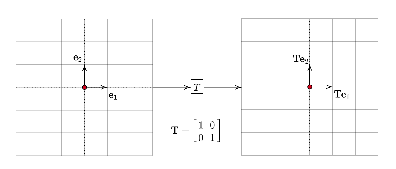
This is not all that interesting. Next:
\[ \begin{equation*} \mathbf{T} =\begin{bmatrix} 2 & 0\\ 0 & 2 \end{bmatrix} \end{equation*} \]
Let us see what this does to the basis vectors:
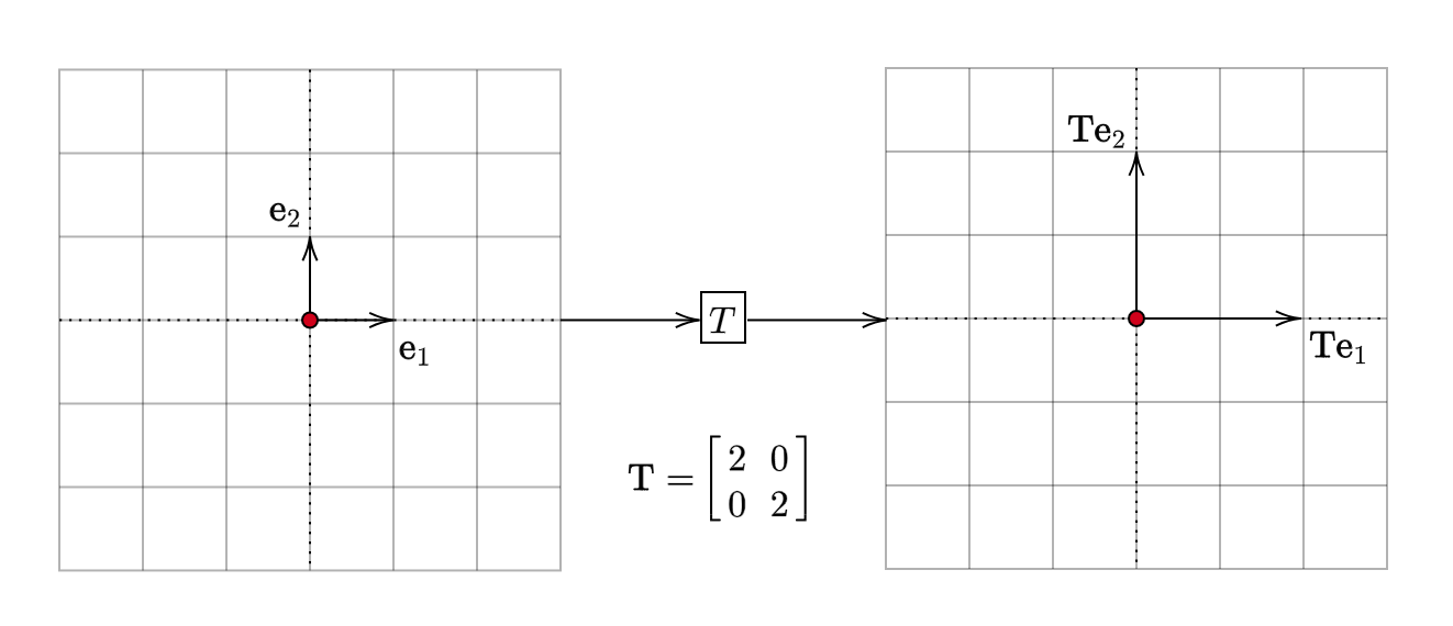
Notice the effect it has. Each vector is scaled. In this case, it is stretched. It becomes twice as long as the input. To see why this is true algebraically, consider an arbitrary vector \(x=\begin{bmatrix} x_{1} & x_{2} \end{bmatrix}^{T}\):
\[ \begin{equation*} \mathbf{Tx} =\begin{bmatrix} 2 & 0\\ 0 & 2 \end{bmatrix}\begin{bmatrix} x_{1}\\ x_{2} \end{bmatrix} =2\cdot \begin{bmatrix} x_{1}\\ x_{2} \end{bmatrix} =2\mathbf{x} \end{equation*} \]
Let us now consider another matrix:
\[ \begin{equation*} \mathbf{T} =\begin{bmatrix} 0 & -1\\ 1 & 0 \end{bmatrix} \end{equation*} \]
The effect it has on the basis vectors is:
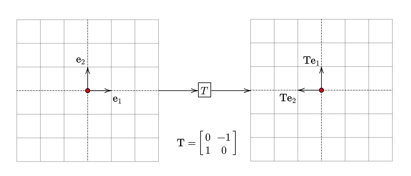
This is a rotation matrix. That is, it rotates the input vector without changing its magnitude. Moving on, let us take up another matrix. This time, let us compose the two linear transformations that we have seen. Composition of linear transformations is equivalent to matrix multiplication:
\[ \begin{equation*} \mathbf{T} =\begin{bmatrix} 0 & -1\\ 1 & 0 \end{bmatrix}\begin{bmatrix} 2 & 0\\ 0 & 2 \end{bmatrix} =\begin{bmatrix} 0 & -2\\ 2 & 0 \end{bmatrix} \end{equation*} \]
What do you expect this matrix to do?
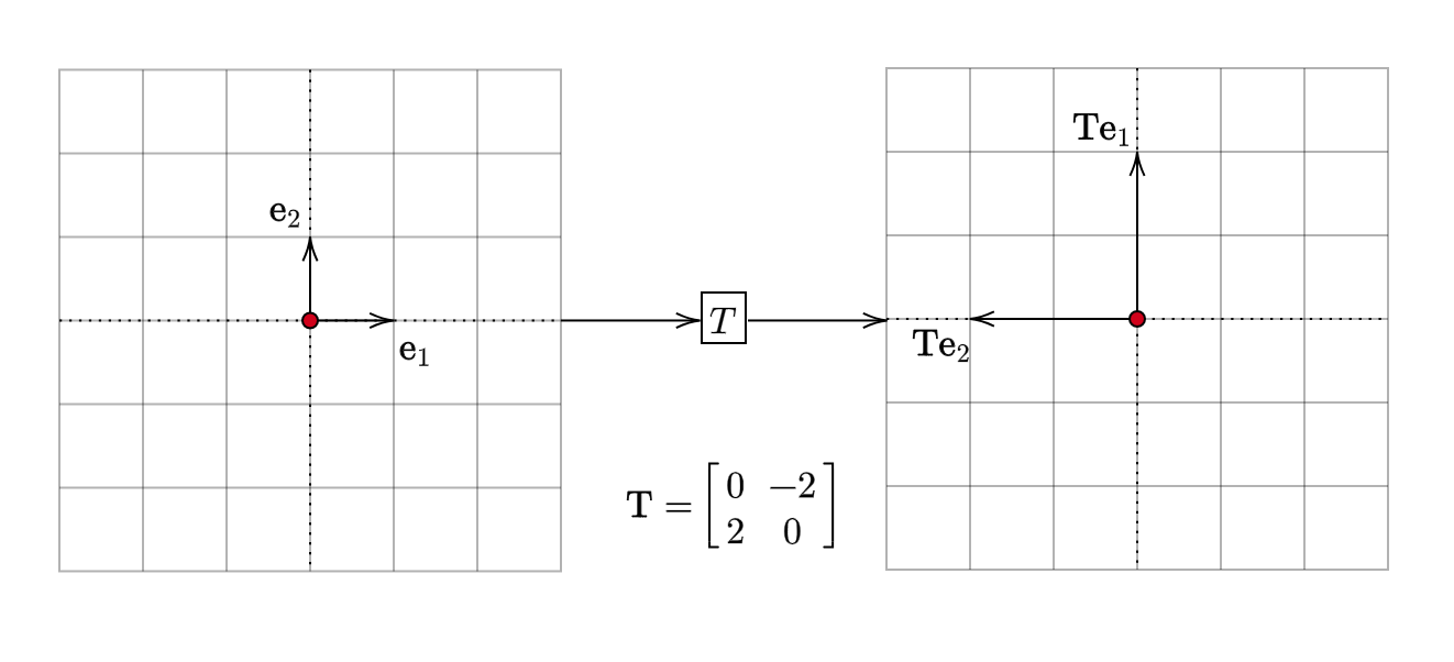
It stretches the vectors and rotates them by \(90^{\circ }\). Note that the two matrices involved in the product are commutative. That is, \(\mathbf{T}_{1}\mathbf{T}_{2} =\mathbf{T}_{2}\mathbf{T}_{1}\). Intuitively, we can see why this is true. We could either stretch a vector and then rotate it (OR) we could rotate it and then stretch it. However, this (commutativity) is not true of any two arbitrary linear transformations. Let us now move to a more complex linear transformation:
\[ \begin{equation*} \mathbf{T} =\begin{bmatrix} 2 & 1\\ 1 & 2 \end{bmatrix} \end{equation*} \]
The effect on basis vectors is:
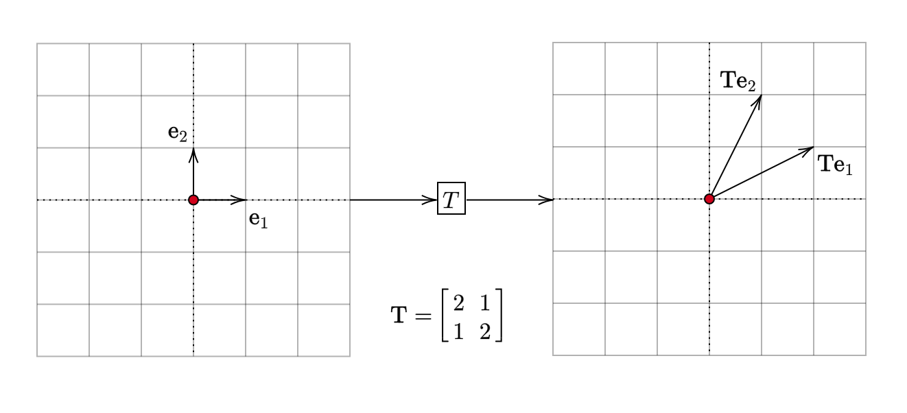
This is not simple rotation or stretching. It is an example of a shear transformation. Now that we have a good idea of what linear transformations do, we are ready to explore the idea of eigenvalues and eigenvectors.
Summary
A linear transformation \(T\) is a linear mapping between vector spaces. The action of a linear transformation on the basis vectors of the domain provides a complete description of what it does to all the vectors in the domain. Every linear transformation corresponds to a matrix. The action of a linear transformation on a vector is equivalent to pre-multiplying the vector with the matrix.